IGEM:IMPERIAL/2006/project/Oscillator/Theoretical Analyses/Results/2D Model5
Introduction
Generalities
- We now study the Dynamical System in its entirety and whole complexity.

Physical interpretation of the equations
- The prey (AHL) production is limited by the limited number of promoters, which can be modelled by a Michaelis-Menten-like kinetics. For very small values of the prey-population (X) the growth can still be assumed proportional to the population (as with Lotka-Volterra). However, for larger populations it becomes constant as the system reaches saturation due to the limited number of promoters.
- The first part of the degradation term of the preys is due to an enzymatic reaction, typically modelled with a Michaelis-Menten kinetics.
- The predator’s growth is the direct result of interacting the preys. All the arguments that bounded the growth of the preys apply to the predators (production is limited by the number of promoters as well). This results in a Michaelis-Menten-like kinetics
- The washout of the chemostat is taken into account
- - it adds dissipative terms to the degradation terms of both preys and predators
- - both dissipative terms are proportional to their respective populations
- The population of the predators is still subject to its natural degradation (proportional to the population) but the term is assumed negligible compared to the washout term
Dimensionless Model
- The complete model comprises 8 variables , which makes its study un-necessarily complex.
- In order to make the important quantities of the model stand out we normalise it by rescaling the X,Y axes and changing the time scale (and in the process end up with 5 variables only)

- The rescaled spatial variables are U=X/ao , V=aoY/co and the time variable is now s=at/ao
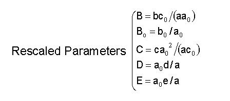
- The parameters of the dimensionless system are linked to the parameters of the previous system as follows:
Basic Results on the Steady Points
The analysis of the whole system remains complex despite the normalisation. Only the most important results are spelt in this section. Anyone wishing to know more about the position and nature of the steady points are encouraged to consult the attached documents at the bottom of the page.
Number of Steady Points
- The system has between 1 and 5 stationary points
- The origin (0,0)
- A second point on the X-axis ((1-E)/E,0) if E<1
- The remaining points are associated with a cubic equation and are not located on any axis
Nature of the Steady Points
- The nature of these steady points (saddle, stable,centre, unstable) varies with the parameters. :*However, the influence of the washout parameters stands out: the larger they are, the more stable the system is.
- Analysis shows that there exist some combinations of parameters for which all steady points of the system are unstable (a necessary condition for the existence of a limit cycle).
Behaviour at Infinity
Importance of the Dissipative Terms
- It is straightforward to show that the dissipative terms –DV and –EU terms prevent the trajectories from going to infinity.
- In particular they prevent the prey-population explosion scenario encountered with the previous model.
General Behaviour
- The system can operate in two distinct modes
- trajectories remain bounded and spin around the steady points of non-zero ordinate
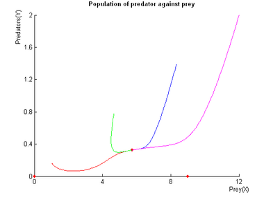
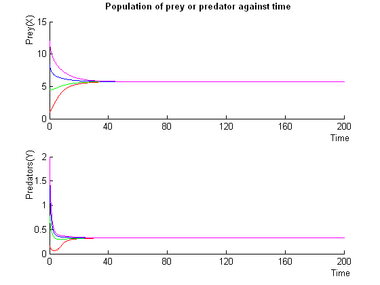
- when at least one of these points is stable, the system stabilises itself at the steady point
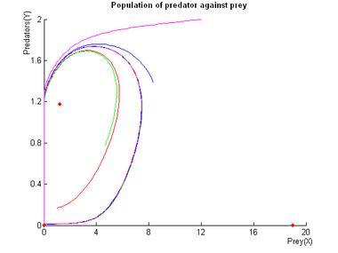
- else we have oscillations around a unique limit-cycle
Typical Simulations
First Mode: Stability
Second Mode: Oscillations
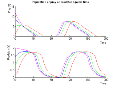
- Note on the Simulations:
- Simulations using different initial conditions are assigned different colors (the open-end of the trajectories is the starting point).
- In the phase diagrams , red dots symbolise a steady points.
Control of the Oscillations
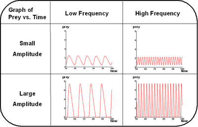
Control of the oscillations is not as simple as with Lotka-Volterra when we take into account the experimental constraints on the model parameters ao,bo and co. Simulations still show that we have good control over the amplitude and total control over the frequency.
No Experimental Constraints
- Let us discuss first the case when we can modify the parameters ao and co.
- Thanks to the analysis of the dimensionless model we can find dimensionless parameters that will yield oscillation (of certain amplitude and frequency).
- Since the scaling along X and Y depends on ao and co it follows that if we can modify these parameters then we can obtain a cycle that is as large along X and Y as we wish. Consequently we can control the amplitude.
- Control of the frequency can be done as usual by multiplying at once the parameters a,b,c,d and e by the same positive value.
With Experimental Constraints
- The model parameters ao, bo and co are all fixed in our model since they are characteristics of the expression of various genes.
- We therefore do not have the freedom to dilate the scales as before: our control of amplitude is as good as our control of amplitude over the dimensionless model.
- The subspace of parameters of the dimensionless model corresponding to oscillation is unfortunately complex. Our rules for modifying the parameters are therefore not as precise as for Lotka-Volterra
- Achieving very small amplitudes
- This is easy. As shown in the detailed analysis attached below, this can be done by choosing D that is small enough so it can oscillate, but large enough so we are very close to the stable regime.
- Achieving Large Amplitudes
- This is trickier. In theory when we decrease the washout term E we should get behaviours that are increasingly similar to those studied in model 4. In particular we could get increasingly close to the prey-explosion mode for well chosen parameters. This suggests that we can amplitudes that are as large as we want.
- Unfortunately we were unable to produce any simulation that justifies this 'hunch'. More work needs doing on the subject of control of amplitude. In the future work section we suggest carrying out a detailed analysis of the entire range in amplitude of the dimensionless model with and without the experimental constraints on the washout.
Simulations
- In the following simulations the amplitude was controlled after setting ao and co to 1 (as with the dimensionless model).
- Control of the frequency was achieved by multiplying at once the parameters a,b,c,d and e by an adequate positive value.
Conclusion
- The 2D Dynamical System models the Molecular Predation System under a reasonable (i.e biologically justifiable) assumption.
- Theoretically we can find combination of parameters for which the system will oscillate around a Unique Limit-Cycle. We can therefore truly speak of a Molecular Predation Oscillator.
- The presence of a Limit-Cycle gives the system a robustness with regards to the choice of initial conditions and experimental accidents that was not present with Lotka-Volterra. In this regards the Molecular Predation Oscillator is an improvement on a pure Lotka-Volterra.
- We have control over a large range of amplitude as well as total control over the frequency of the oscillations. We have conjectured that the control over the amplitude is actually total as well.
Appendices
- A more detailed analysis of the system was made by Matthieu. Please consult it if you have any questions on the results on this page.