IGEM:IMPERIAL/2006/project/Oscillator/Modelling/LV
MODELLING THE OSCILLATOR AND ITS COMPONENTS:
Lotka-Volterra Modelling
First, we considered the Lotka-Volterra model and it's consequences before actually modelling our system because of the similarities.
- Click File:Oscillationmodelv2.xml to access the SBML file which we used to simulate the Lotka-Volterra model on CellDesigner 3.2.
- Realistic Values to be used in descriptive models.
- Analysis of LV model
- Document on how to effectively extract parameters from Michaelis Menten model, by Matthieu Bultelle
Theoretical Analysis
Analysis of ODEs of the given system - mathematical approach to study and characterise the systems behaviours
Aim:
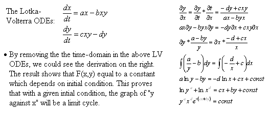
- To have a basic understanding of the Lotka-Volterra (LV) Equation on how it resulted in a unstable oscillation
- To study to the key parameters for their effects on the amplitude and the frequency of output oscillation
- Further modify the LV equation to model our real system
- Further study the modified model based on LV model
- Propose a set of realistic parameters which will achieve the system design aim
Progress:
<showhide>
1. Analysis report of the past progress --31/07/06
- We have underestimated the complexity within the simple lotka-volterra model
- However, we did have a basic understanding of the LV ODEs, the following is the abstract of above document __HIDER__
<hide>
- limit cycle
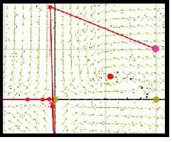
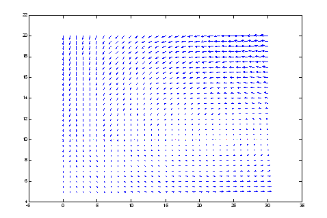
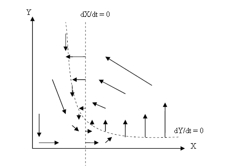
- vector field - a powerful way to represent the system behaviour
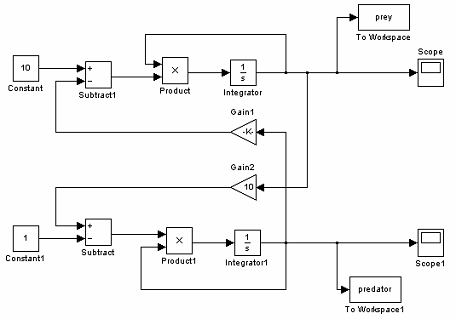
- Control modelling - using simulink in Matlab
- use control modelling technique to model and simulate the system
- from the above model, we are able to change the parameters and initial condition to study the behaviour of the system
- we have found that the LV system is not as easy as expected, in fact, it is very sensitive to noise, any small perturbations will trigger the system into a different cycle
- It is also impossible to characterise the effect of changing paramenter on output waves' frequency and amplitude.
</hide></showhide>
- However, the result from Simulink and matlab programming is not promising, the output seems to be noisy. Simulink is very complex itself, and we fail to apply any advance control method to simplify our system, hence the method of using Simulink is discarded
2. Back to simplicity -- another new matlab programme has been done, we just used ode23 to solve LV differential equations
Objective:
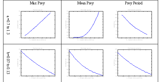
- To avoid the complexity, we will only vary one parameter at a time, to find out about the resultant change on the output period and frequency
- Since as mentioned above, the system behaviour might be totally different, here we are going to study a typical set of parameters, and hopefully could use this approach to create a template to study our real system paremeters.
Result:
<showhide>
-- click here for the first report --02/08/06
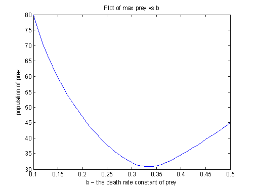
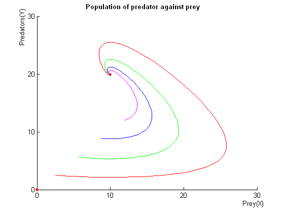
- This document shows graphs of magnitude of output against the changing of parameters. A typical graph: __HIDER__
<hide>
</hide></showhide>
<showhide>
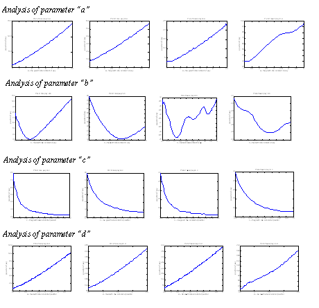
-- click here for the second report --04/08/06
- This document is an improvement over first report. A general trend can be concluded from this documents, a few chosen graphs are shown here. __HIDER__
<hide>
</hide></showhide>
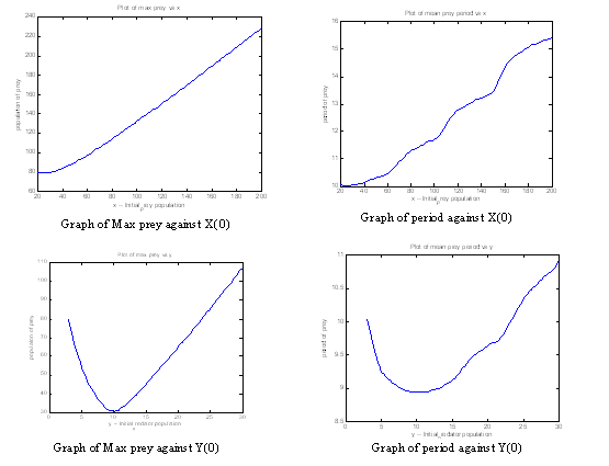
<showhide>
-- click here for the third report --07/08/06
- This document studies the effect by changing the initial condition, a few chosen graphs are shown here. __HIDER__
<hide>
</hide></showhide>
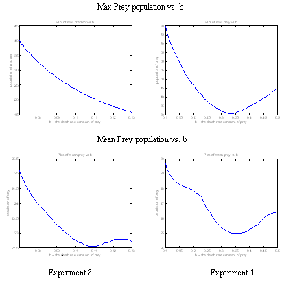
<showhide>
-- click here for the fourth report --07/08/06
- This document verify the local behaviours of parameters by using a smaller range. __HIDER__
<hide>
</hide></showhide>
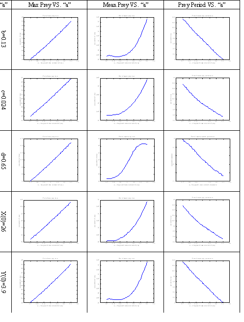
<showhide>
-- click here for the fifth report --10/08/06
- Further verify the local effects of a single parameter while setting the rest of parameters to a different value. Presentation of results has changed to a table form format. __HIDER__
<hide>
</hide></showhide>
<showhide>
-- click here for the sixth report --10/08/06
- Once we confirmed the local behaviour and choose a set of parameters, we ran a stress analysis to study how sensitive the system is to each parameters. Example:__HIDER__
<hide>
</hide></showhide> Conclustion:
- We have done the numerical analysis with a given set of ODEs and parameters
- Now we should be able to analyse, predict and choose a set of parameters to achieve our system design aim.
- However, as the ODE system will become more and more complicated, if possible, we need a theoretical approach to understand what the system should behave before analysing them numerically.
3. Jacobian anaylsis of stationary point for stability of oscillation. click here --04/08/06
Method to determine the stability of a stationary point:
- Formulate the differential equations.
- Find out about the stationary point by setting the differential equations to 0.
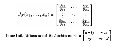
- Form Jacobian matrix using partial differentiation on differential equation.
- Substitute the stationary point value into the matrix and obtain its eigen value.
- Determine whether the stationary point is stable.
<showhide>
The above document shows how a matlab programme is used to generate required data. __HIDER__
<hide>

- Now we have a Matlab tool to study a given ODEs
<showhide>
4. Introduction to analysis of the 2-D ODEs. click
here --14/08/06
- Step by step analysis of pure Lotka-Volterra ODEs, detail explanations of every step taken __HIDER__
<hide>
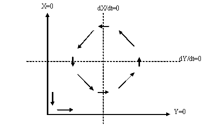
- stationary point: points when the system reach a steady state (equilibrium)
- Jacobian matrix: best linear approximation to a differentiable function near a given point, can be used to determine whether these points are stable
- Eigen value of Jacobian matrix: The sign of the real parts of eigenvalues will determine whether the given stationary point is stable.
- Hence we can use Trace and determinant of a Jacobian matrix to determine the stability of 2-D ODEs
- Vector Field Representation: A powerful numerical method to help us visualise the stability of a give point.
- Thus we have define our approach to study a give ODEs with appropriate explanations.
</hide></showhide>
--revised version 1 click here --21/08/06
- An improved version, rephrased various definations, and added the reason for using eigen-values to determine the stability of a stationary point.
<showhide>
5. Study and Characterisation of a limit cycle. click here --06/09/06
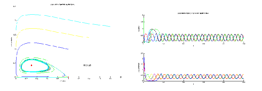
- Showing a typical ODEs that will result in a nice limit cycle; this should be our aim of the modelling. There is also a short discussion on how to characterise the limit cycle. Graph __HIDER__
6. Stability analysis of modified Lotka-Volterra systems
<showhide>
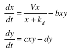
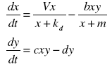
- The pure Lotka-Voleterra model is too ideal to achieve, after our careful analysis, we think that our model should be modified similar to Michaelis-Menten __HIDER__
<showhide>
-- Version 1, production of the prey is modelled by pseudo Michaelis-Menten kinetics click here --16/08/06
- After the analysis, there are two stationary points [0, 0]&[d/c, V*c/b/(k*c+d)], first being unstable, second being stable __HIDER__
<showhide>
-- Version 2, productions of the prey and predator are modelled by pseudo MM kinetics click here --21/08/06
- There are also two stationary points
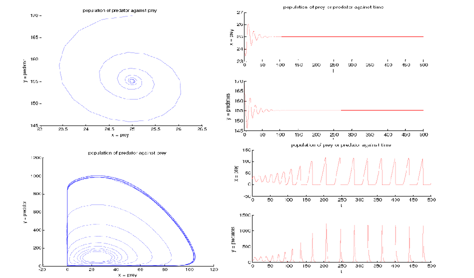
- The following graphs shows case when k<m & k>m __HIDER__
<showhide>
-- Version 3, production and death of the prey is modelled by pseudo MM kinetics click here --06/09/06
-- Version 4, Combination of Version 1 2 3 click here --06/09/06
-- Version 5, with E, click here
Further Study of the complicated modelling of Version 4
Specail thanks to Matthieu Bultelle for all the mathematical analysis of this model!
-- Trial 1, by defining R=B*C/D to simplify stability analysis, click here for analysis and click here for appendix of full-size graphs --06/09/06
-- Trial 2, interesting cases of trial 1, click here for cases of R=1 and click here for an interesting nice limit cycle --06/09/06
-- Trial 3, by re-defining R=C/D for better system analysis click here for analysis and click here for appendix of full-size graphs --07/09/06
List of templates designed by Matthieu Bultelle:
-- Part 1, Dynamic Analysis of a system, click here
-- Part 2, Poincare Analysis for limit cycle, click here
-- Part 3, Theoretical Model Analysis, click here
-- Part 4, Presentation of Results, click here
Template for analysing dynamical system : IGEM:IMPERIAL/2006/project/modelling_template
A powerful Java Applet
<HTML> <HEAD> <TITLE>Molecular Prey-Predator-System</TITLE>
<LINK REL="stylesheet" TYPE="text/css" HREF="style.css">
</HEAD> <BODY>
Molecular Prey-Predator using JOde
<APPLET code="com/rychlik/jode/JOdeApplet.class" NAME="JOde" width=650 height=750 archive="http://openwetware.org/images/a/a3/JOdeApplet.jar" mayscript="true"> <PARAM NAME="isframed" VALUE="false"> <PARAM NAME="background" VALUE="c0c0c0"> <PARAM NAME="autonomous" VALUE="true"> <PARAM NAME="min1" VALUE="0"> <PARAM NAME="max1" VALUE="50"> <PARAM NAME="min2" VALUE="0"> <PARAM NAME="max2" VALUE="1"> <PARAM NAME="variable0" VALUE="t"> <PARAM NAME="equation0" VALUE="a=1;a0=1;b=5;b0=0.5;c=0.01;c0=1;d=0.02;e=0.01"> <PARAM NAME="variable1" VALUE="X"> <PARAM NAME="variable2" VALUE="Y"> <PARAM NAME="equation1" VALUE="a*X/(a0+X)-b*X*Y/(b0+X)-e*X"> <PARAM NAME="equation2" VALUE="c*X*Y/(c0+X*Y)-d*Y"> <PARAM NAME="initconds" VALUE="40,1;10,0.2"> <PARAM NAME="showinitconditions" VALUE="true"> <PARAM NAME="showpoints" VALUE="false"> <PARAM NAME="showslopes" VALUE="true"> <PARAM NAME="showaxes" VALUE="true"> <PARAM NAME="minparameter" VALUE="0"> <PARAM NAME="maxparameter" VALUE="2000"> <PARAM NAME="parametersegments" VALUE="20000"> <PARAM NAME="algorithm" VALUE="RK4"> <PARAM NAME="label" VALUE="Molecular Prey-Predator"> </APPLET>
a=1;a0=1;b=5;b0=0.5;c=0.01;c0=1;d=0.02;e=0.0
Instructions on using the JOde Applet</A>
Using the applet written by: <A HREF="http://alamos.math.arizona.edu/">Marek Rychlik</A> </BODY> </HTML>
