Beauchamp:NIRS
Beauchamp Lab wiki
|
Eswen Fava's NIRS Manual
Probe Creation:
- 3.2cm from source to detector for adults (note absorption is 2/3 the distance of source to detector)
- 2 cm from source to detector for infants
- 2.5 cm from source to detector for children
- [Munster T2T-Converter (3D Version)[1]] (does not open in new window!)
- Tools that are helpful:
- simple: compass, superglue (with brush), hand single hole punch, drill bit to go through plastic
- speciality: face-lift compression garments, scuba caps, soccer header headband (temporal probe),
- online vendors: McMaster-Carr - nylon machine screws, panhead 1/4" in length
Experimental Design:
- Keep in mind Hemodynamic Response Function properties when designing an experiment using NIRS
- e.g., Infant experiments (Bortfeld, Fava & Boas 2009) duration of baselines: 10 seconds, duration of stimuli: 20 seconds
Hemodynamic Function (HRF):

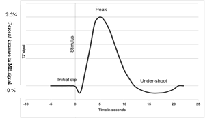
- After the onset of the stimulus, a small decrease in MR signal is observed, caused by the fact that oxygen from the blood is used, but that the blood supply is not yet altered. This makes that the concentration deoxyhemoglobin rises and that the MR signal is more disturbed.
- Shortly after this initial dip, the signal rapidly begins to rise due to the supply of more and more oxygenated blood. There is more supply of oxygenated blood than is necessary and this gives an increased MR signal till the end of the stimulus. A few seconds after the end of the stimulus the signal rapidly decreases to end, via a post-stimulus undershoot, at its normal level.
- The post-stimulus undershoot is caused by the fact that the cerebral blood flow is more locked to stimuli than is the cerebral blood volume. The resulting increase in blood volume leads to a decrease in MR signal. Picture is obtained and adapted from the website of Radiopaedia [79].
- To find the small increase in MR activity due to the stimulus, usually the General Linear Model (GLM) is used. With this method the activity due to the presented stimulus is modelled by convolving the time-course of the stimulus presentation with the hemodynamic response function. In the next step the correlation between the model and the time course of the MR signal at each voxel or region is calculated by using linear regression. The result is a regression coefficient (r) and a p-value for each voxel or region. The p-value indicates how likely it is that the correlation between the GLM and the time course of the signal can be explained by chance instead of the stimulus."
Taken from mst.nl http://www.mst.nl/neurochirurgie/Onderzoek/tinnitus.doc
Checking Laser Reading Power Levels:
(Note: you CANNOT see 830nm, you CAN see 690nm (appears red))
- all lasers of same wavelength should be in the same range (e.g., all 690 lasers should be between 13.01 and 13.9)
- adjust lasers with small screwdriver.
- when you unscrew the detector fibers from the machine, turn the machine off completely before you do so. Otherwise, you expose the receiver to light and may burn it out.
- when using power meter to measure from the laser
- 690nm should read at 13mW or 12.5mW
- 830nm should read at 10mW
- when using power meter to measure from the probe end of your fibers, expect your fibers to lose between 30 and 50% of the light
- 690nm should be about 8.45
- 830nm should be about 6.45
Checking your Fibers:
- If you move your fibers around a lot, or exchange one set for another consider frequently checking them once per month
- You can also check your fibers by holding the laser end up to an incandescent bulb and holding the emitter’s probe end to the wall. The light should form a whole circle.
- Be sure to look at 1 wavelength at a time
- When you receive new fibers, hook them up to the 690nm lasers and hold them up to the wall to check for the whole circle pattern
- If you don’t see that pattern, epoxy or broken fiber optics could be to blame. Send them back!

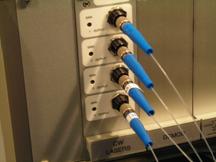
Checking your Lasers (see picture at right):
- Turn Laser 1 ON (690nm)
- Turn all other Lasers OFF
- Probe ends of fibers are facing a wall
- Remove fiber from Laser 1 690 source - watch for any changes in amplitude or signal quality for detectors 1&2
- Repeat for all source-detector pairs (be sure to turn ON the laser you want to investigate, and OFF the remaining lasers)

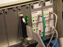
Checking your Detectors (see picture at right):
- Turn ON all lasers
- Unplug ALL detectors
- Plug in detectors one at a time and note any changes in the amplitude or signal quality change
Checking to see which Detectors your Sources go to:
- Use a phantom head, or wrap a blanket in a tight ball
- Put probe on phantom
- Turn ON a source (e.g., turn on Laser 1)
- With a source on, REMOVE detectors 1 by 1 (leave the previous detectors unplugged as you continue) - note any changes in movement, or lack of movement from the detectors.
- Note if pre-clipping gain light is on or not for each of the detectors
- Plug all detectors back IN, turn OFF source 1, Repeat steps 3 and 5, cycling through your sources. Continue this process until you have gone through all of your sources.
Checking to see which Sources your Detectors go to:
- Use a phantom head, or wrap a blanket in a tight ball
- Put probe on phantom
- Turn ON all sources (e.g., turn on Lasers 1, 2, 3, 4)
- With all sources on, REMOVE only detector 1
- Note any changes in movement, or lack of movement from the remaining plugged in detectors as you do this
- Note if pre-clipping gain light is on or not for each of the detectors
- Make sure all detectors are plugged IN, keep ALL sources ON, repeat steps 3 through 5, cycling through your detectors. Continue this process until you have gone through all of your detectors.
Data Analysis in Homer (version 08-11-18):l
- In this version, homer is an executable.
- A new version of homer was made available at the fNIRS conference 10/15/10, which runs on matlab
Importing a file:
- File > Import data to current session > select .nirs data file
- Enter session identifier: put anything here, it doesn't matter (e.g., "a" or "1")> "ok"
Filtering Menu: (see filtering button)
- LPF = low pass filter - this depends on your experiment.
E.g., For a 20s on / off paradigm, the period is 40s --> frequency = 1/period --> f = 1/40 = 0.025Hz We want the cut off below this, so you might try 0.01
- HPF = high pass filter that removes frequencies typical of heartbeat or respiration, etc - for adults this is 0.5 - for infants try 0.8
- "update file"
- note: nSV motion is a PCA filter for motion
- Data Display Controls: here you can see the optical signal with various amounts of filtering, the further down the menu you go, the more filtering takes place, raw intensity is good ot look at to see the intensity unites (Arbitrary Units) that should match the units you noted when you recorded the signal.
- Cov. Reduced dConc is what we usually look at for the stimuli (that's what EASYNIRS shows you)
- Make sure that your probe geometry is appropriate - xs are emitters, os are detectors
Averaging Menu: (see averaging button)
- HRF Timing: This shows you the average in relation to you stimuli marks
- (e.g., preTime -5; postTime 30) When you hit "calculate average" you'll see 5 seconds before your stimulus mark and 30 seconds after your stimulus mark
- "Show stim:" If you have marked stimuli as you recorded your NIRS signal
- To deselect stimuli, click on them so that vertical green line in the main window is dotted and red. If the dotted line is red then that stimulus mark will be included in your average
- "User stim": You can also put in stimulus marks by entering values in seconds in the "user stim" window between the square brackets. Once you're done entering values, hit "user stim" and they should show up as vertical green lines in the main window.
- "Display controls" You can toggle between different views of the optical data here, just as in the filtering tab. The further down you go, the more signal processing takes place.
- Cov. Reduced dConc is what we usually look at for the stimuli (that's what EASYNIRS shows you)
- You can also copy the graph in the main window and use a tracer to see the exact data points. (Right click on your mouse when you have your mouse in that window, make new figure.)
- You can toggle between the Filtering and Averaging menu by pressing the buttons at the bottom of the screen.
ROI analysis (tab on right hand side of homer window)
- Here you can look at HbO (red) , HbR (blue) and HbT (green) hit" calculate HRF for ROI"
- A session is essentially 1 window to analyze a bunch of babies. You can open more than 1 session at a time, but I have found homer crashes after more than 10 babies anyway, so I haven't used this option.
Notes from fNIRS Conference (Oct 15-17, 2010, Boston): http://www.nmr.mgh.harvard.edu/fNIRS/index.html
- Report both HbO and HbR (An increase in HbO should also correspond to a decrease in HbR)
- Use a phantom head and report those data prior to experiment data
- Use of a systemic data in order to eliminate that noise from the NIRS signal
Issues in the field to work on/ think about:
- Perhaps make analysis code publicly available?
- Use of better statistics than just area under curve/ time to peak, etc
- Standardization of instruments
- Standardization of probes
Links:
North America:
- Northwestern University (Sue Hespos): http://groups.psych.northwestern.edu/infantcognitionlab/
- Rochester Group NIRS data analysis (Dick Aslin): http://www.bcs.rochester.edu/people/aslin/mcdonnell/NIRS.html
- Stanford (Cui Xu): http://www.stanford.edu/~cuixu/
- Stanford(John Oghalai): http://med.stanford.edu/ohns/research/labs/labs_oghalai.html
- Texas A&M University (Teresa Wilcox): http://psychology.tamu.edu/Fac_Ext.php?ID=35
- U Connecticut (Heather Bortfeld): http://bortfeld.psy.uconn.edu/
- University of Montreal:
- University of Pittsburgh (Ted Huppert): - Homer Software http://www.pitt.edu/~huppert1/Huppert_UPitt/Lab_Publications.html
- U Toronto (Missassauga)(Laura-Ann Petitto): - NIRS-SPM Software http://www.utsc.utoronto.ca/~petitto/
- U Toronto (Toronto): Physiology:
- TechEn: http://www.techen.com/
Europe:
- Berlin NeuroImaging Center: http://www.berlin-neuroimaging-center.de/publications
- Karolinksa Institute, Stockholm: http://ki.se/ki/jsp/polopoly.jsp?l=en&d=34984
- SISSA, Trieste: http://www.sissa.it/cns/lcd/jacques.htm
- University of Chieti, Chieti (Italy):
- UCL Group: http://www.ucl.ac.uk/medphys/research/borl/nirs
- University Hospital, Zurich:
- University of Helsinki:
- University of Munich (Dept. Neurology & Psychiatry)
- University of Padua, Padova:
- University of Paris - Descartes (Psychological Perception Lab), CNRS, ENS-Paris : http://lpp.psycho.univ-paris5.fr/speech.php
- University of Wurzburg, Clinical Center: http://nervenklinik.uk-wuerzburg.de/forschung/arbeitsgruppe-genomische-bildgebung/forschungsthemen/nah-infrarot-spektroskopie.html
- Zurich Neuroscience Center: http://www.neuroscience.ethz.ch/research/biomedical_technology/wolf
Japan:
- Chuo University (Tokyo):
- Hitachi, Ltd (Tokyo):
- Kawaga University (Kawaga):
- Kanazawa University (Kanazawa):
- Tokai Gakuin University, Japan
- Tohoku University,
- University of Tokyo: