BME100 s2018:Group1 W0800 L6
OUR TEAM
 |
 |
 |
Bayesian Statistics
Overview of the Original Diagnosis System
Ten groups were given two patients to diagnose. Each group had three samples of each of their patients, for a total of six samples. This technique, PCR, allows the desired genetic sequence to be amplified and was visually displayed by means of SYBR Green 1. The amount of green present in the patient's samples were compared to the positive and negative controls which revealed if the patient's samples were either positive or negative. For this lab, the groups were tasked to compare the results of the patient's samples against a positive and a negative control. Error was minimized by having three samples from each patient. For the groups to accomplish this, one or two individuals were focused on the ImageJ image processing software, which was able to filter out the green light. By comparing the concentration of green in each droplet to the controls, the results were determined to be either aligned or not aligned with the positive or negative. Additionally, each sample was digitally analyzed three times and averaged to further minimize error. The majority of groups received conclusive data, and this data is broken down in the above charts. Only Group 7 had an inconclusive test for patients, with a total of 14 patients having a negative result, 5 having a positive result, and one group unable to provide test results, neither inconclusive nor negative nor positive. From this, there were 14 negative diagnoses and 6 diagnoses. every positive and negative result corresponded to a diagnosis and not diagnosis respectively, with the inconclusive result also receiving a diagnosis.
Table 1
| Variable | Description | Numerical Value |
|---|---|---|
| A | Positive final test conclusion | 0.25 |
| B | Positive PCR reaction | 0.25 |
| P(B,A) | Positive PCR given positive final test | 0.933 |
| P(A,B) | Positive final test given positive PCR | 0.933 |
Table 2
| Variable | Description | Numerical Value |
|---|---|---|
| A | Negative final test conclusion | 0.7 |
| B | Negative PCR reaction | 0.72 |
| P(B,A) | Positive PCR givne negative final test | 0.95 |
| P(A,B) | Negative final test given positive PCR | 0.93 |
Table 3
| Variable | Description | Numerical Value |
|---|---|---|
| A | Will develop disease | 0.3 |
| B | Positive PCR reaction | 0.25 |
| P(B,A) | Positive PCR reaction given that disease will develop | 0.6 |
| P(A,B) | Disease will develop given positive PCR reaction | 0.72 |
Table 4
| Variable | Description | Numerical Value |
|---|---|---|
| A | Will not develop disease | 0.7 |
| B | Negative PCR reaction | 0.7 |
| P(B,A) | Negative PCR reaction given that disease will not develop | 0.857 |
| P(A,B) | Will not develop disease given negative PCR reaction | 0.857 |
What Baynesian Statistics Imply
Table 1 describes the sensitivity of the system regarding the ability to detect the disease SNP. Table 2 describes the specificity of the system regarding the ability to detect the disease SNP. Table 3 describes the sensitivity of the system regarding the ability to predict the disease. Table 4 describes the specificity of the system regarding the ability to predict the disease.
Three examples of sources of error are the difficulties of micropipetting, the difficultly of achieving complete darkness, and the shifting of the smartphone camera through the experiment. Firstly, there would frequently be residual liquid after fully releasing the micropipette tip. This would make the concentration of all the droplets slightly lower than they should be, and because this amount was slightly different for each sample. Secondly, the photos of each droplet were taken in a fully lit building, and only the apparatus was covered by a small black box. Although this covered much of the light of the room, this did not completely conceal the light, and the results would have been more accurate without its presence. Thirdly, the distance between the smartphone and the stand was maintained as close as possible during the experimentation however in order to send the images to the computer for digital analysis and in order to reset the timer on the phone, it was shifted slightly closer and closer to the droplet.
| Consumables: plastics, pipettor, and reagents (PCR mix, primers) | The OpenPCR machine and software | The Fluorimeter system (including slides, stand, etc.) |
|---|---|---|
Strength:
|
Strength:
|
Strength:
|
Weakness:
|
Weakness:
|
Weakness:
|
Consumables Kit Improvement Notes:
Bubble wrap, label everything and it all comes in one package, so it cannot be lost, color code the primers and tubes to indicate where everything goes to eliminate cross contamination and accidents.
Hardware: PCR Machine Improvement notes:
Double the number of slots for more trials and experiments
Hardware: Fluorimeter Improvement Notes:
Attach the phone stand to a fluorimeter stand to keep the distance constant throughout the experiment; able to adjust distance away from fluorimeter, height, locks phone into place
What Bayes Statistics Imply About This Diagnostic Approach
Intro to Computer-Aided Design
Feature 1
The consumables used in the lab will mostly remain the same for our improved fluorimeter design. The same size tubes and the same micropipettor will be used. Also the glass slides will be used again with our fluorimeter. In addition all of the solutions will be the same and used with a very similar procedure to the original PCR and Fluorimeter set up. The difference with our materials would be to add a color coding of the test tubes and the solutions that will be transferred. This would allow for easy transfer of solutions with less chance of error in mixing up the proper location of each solution. There will be a colored circle on the side of each PCR tube to indicate which solutions are to be added. Overall all of the consumable materials will be used in the same manner as they were previously.
Feature 2
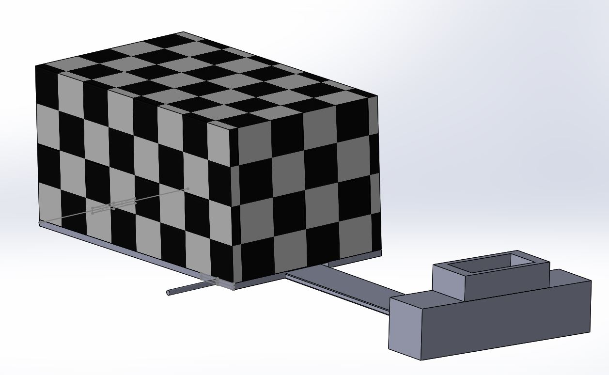
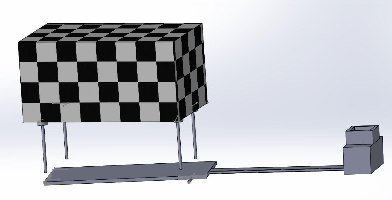
The new and improved fluorimeter system is a simple, easy to use device that will improve the quality of images and results. This is accomplished by a new design in the camera holder that will securely hold the camera in place with a constant force spring. It will also have a sliding ruler connecting to the camera system and the fluorimeter device. This slide will allow the distance between the camera and water droplet to be measured accurately. Once the desired distance is found a screw tightens the camera's case to the slide, holding it securely in place throughout all the trials. This allows the distance to be constant through the entire experiment and the measurements along the slide allow the user to return the camera to the proper distance if it is ever needed from any accidental bump or other mistake in moving the camera. In addition to the distance from the camera and droplet the new fluorimeter also includes a feature to adjust the height of the fluorimeter to match the camera height. This is accomplished by unclipping four clamps on four bolts which are stored in the fluorimeter. The machine can then be lifted, and the clamps re-clip to keep the fluorimeter at the desired height.
The images below represent the new devices. The black and white checkered box represents the fluorimeter. The first image shows the device with the ruler fully out, the bolt screwed in to keep the glider in place, and the constant force spring at a phone's length. The second image shows the fluorimeter with the rising action.

