Analyzing GRNmap Output Workbooks Using Multiple Regression and SPSS
This page outlines how to perform multiple regression analyses in SPSS to analyze data from GRNmap output sheets. Specifically, the protocol written below was used to identify determinants of node MSE:minMSE ratio in db1-db6 by running models in which the aforementioned parameter was the dependent variable. Independent variables included optimized parameters generated by GRNmap (optimized production rate, optimized threshold b), degradation rates, transcription factor expression changes, and graph statistics. The results of this analysis can be found here.
Note: The instructions below were written using SPSS Statistics Version 21.
Step 1: Preparing the Data for Input into SPSS
Before beginning, select the variables you would like to analyze. This process includes designating a dependent variable, selecting possible predictors of this variable (i.e. independent variables), and coming up with a priori hypotheses regarding what relationships you expect to find between the dependent variable and predictors in your regression model. Be sure to write these down. Finally, decide which gene regulatory networks you would like to study.
For each network, create a new excel file where you will compile all of the variables to be analyzed. Compiling this data may be facilitated by creating multiple sheets within a single excel workbook. However, all of the variables to be included in the final multiple regression analysis must be present in a single sheet, which will allow easy export of the data into SPSS. In this final worksheet, each variable to be analyzed should be provided its own column. Although transcription factor IDs should be included for reference, they ultimately will not factor into the multiple regression analysis.
Once all of the variables have been compiled in a single excel worksheet, label that worksheet (e.g. add the suffix _for-SPSS). Then save and close the excel file prior to opening SPSS.
Step 2: Generating an Initial Multiple Regression Model
Launch SPSS, allowing the program several minutes to load. To open the excel file containing the data to be analyzed, navigate to File-> Open-> Data... A window will open prompting you to designate the path to your file. Navigate to the folder containing your file. By default, only .sav files will show up in the selection window. Change the file types displayed to "All Files" or "Excel" so that your excel file will be visible. Once it is, select the file and then click "Open". Another window will open asking you to designate the worksheet containing the data you would like to import. Select the appropriate worksheet name from the drop down window and click "OK". This will open your file in the SPSS data editor. Note that variable names and number formatting may be altered in the import process. To edit this formatting, navigate to the "Variable View" tab visible at the bottom left corner of the data editor. Although most of the formatting options are only for aesthetics, it is critical to check the "Measure" column to select the appropriate data type for each variable. Specifically, all numerical data used in multiple regression analyses should be input as "Scale". Although ordinal data can also be used, scale data is preferred. Often times, integer data imported into SPSS will be incorreclty labeled as nominal data. Be sure to correct any such errors before proceeding.
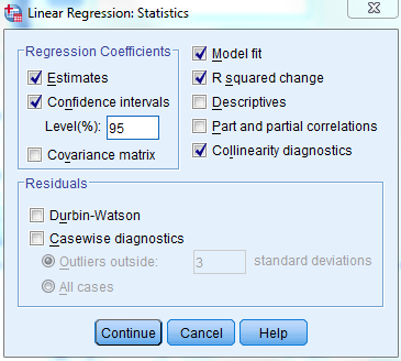
Once all of the data is formatted appropriately, it is time to generate the first multiple regression model. To do so, click on Analyze-> Regression-> Linear... This will open a window prompting you to specify the dependent and independent variables in your regression model. To do so, click on the measure in the column on the left and then click the arrow to the left of the category the variable belongs to (Dependent or Independent). Doing so will import the variable into the model. Before proceeding, click on the "Statistics..." button to customize your regression model outputs. I recommend entering the following settings:
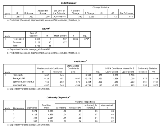
Once you have customized the regression parameters to your liking, click "Continue" to close the settings menu and then click "OK" in the original regression window to run the model. The model results will promptly be returned in the SPSS viewer window. A sample output is shown below:
Step 3: Guidelines for Creating a Final Model via Backward Selection
Although there are many methods for selecting the best regression model (including having SPSS automate this process), I recommend manually performing backward selection. To do so, start off by including all possible predictor variables in your original model. The model summary is likely to have a high "R square" value given that many different predictors were integrated into the model. However, many of the individual model coefficients will be insignificant, which is taken into account by the "Adjusted R Square" goodness of fit measure. When performing backward selection, you will remove independent variables with insignificant model coefficients one at a time until a model containing only significant coefficients is left behind. The purpose of this selection process is to produce a statistically significant multiple regression model that can predict variance in the independent variable, which is measured by the "Adjusted R Square" metric (values closer to 1 indicate better model fit).
When evaluating the original multiple regression model, assess the following criteria to determine which independent variables should be removed:
- Covariance
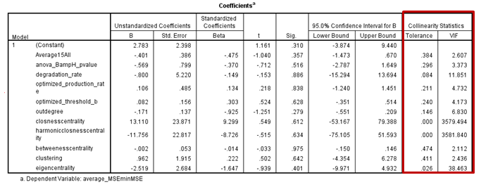
- Independent variables included in the model may be correlated to one another, or covary. If so, this relationship may interfere with the multiple regression model's validity and accuracy. Thus, it is important to screen the "Colinearity Statistics" reported by SPSS for high values (generally values >5 are problematic).
- When a predictor is found to covary with another independent variable(s) in the multiple regression model, those variables must be scrutinized to determine which should be removed. Generally, it is thought that colinear variables capture similar information, and thus can be used interchangeably as predictors in multiple regression models.
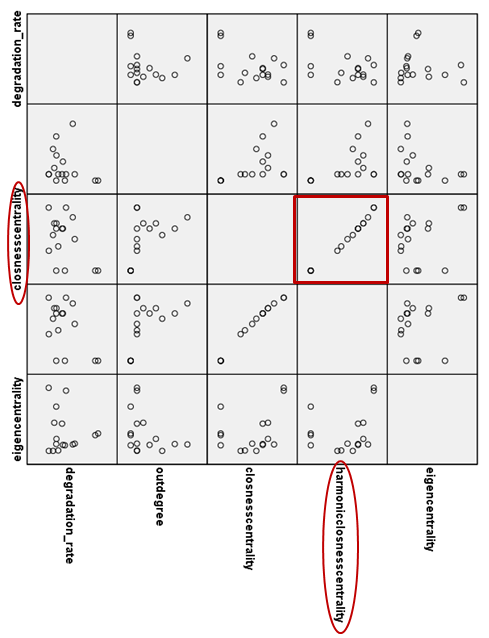
- To visualize how a colinear variable in your model is related to the other independent variables, it is useful to generate a matrix of scatter plots. To do so, navigate to Graphs-> Legacy Dialogs-> Scatter/Dot... In the resulting menu, click on the "Matrix Scatter" option and then select "Define". This will open the Scatterplot Matrix window, where colinear variables can be imported as "Matrix Variables" for analysis. Once the variables in questions have been defined, click "Okay" to generate the matrix of scatter plots. Variable names will be listed on the x and y axes. Review the matrix for scatter plots that exhibit a linear pattern. The variables plotted in these scatter plots are said to be colinear, and one of them will have to be removed. A sample scatter plot matrix showing two highly colinear graph statistics, closeness centrality and harmonic closeness centrality (Colinearity Statistics: Tolerance >0.0003, VIF >3500), is shown below.
- Once two colinear predictors have been identified, it must be decided which should be removed. In making this decision, there are several important points to consider. First, consider your a priori hypotheses. If you reasoned that one of the colinear variables would be a significant predictor in your model, you may want to keep it. Instead, discard the other colinear variable from the model. Alternatively, if you did not make predictions about either independent variable, then determine how each of the predictors correlates to the dependent variable on its own. This can be done by creating individual scatter plots relating each predictor to the dependent variable and determining the R Square value associated with linear trendlines fit to each graph. The predictor that is best correlated to the dependent variable should be kept in the model.
- Once a colinear variable has been selected for removal, rerun the multiple regression model and exclude that variable. This can be done by selecting the appropriate name from the Independent(s) box in the Linear Regression window and clicking the left-facing error next to that box. Then click "OK" to run the new model. Now assess the new colinearity statistics and repeat the above steps until none of the included independent variables are listed as colinear.
- Coefficient Significance and Confidence Intervals
- Now that any colinearity issues have been resolved, begin removing the independent variables one by one that have the least significant coefficients. Insignificant coefficients have "Sig." values >0.05 and 95% confidence intervals that straddle zero (e.g. -1.240, 1.451). Iterate this process until only significant coefficients (Sig. <0.05) remain in the model.
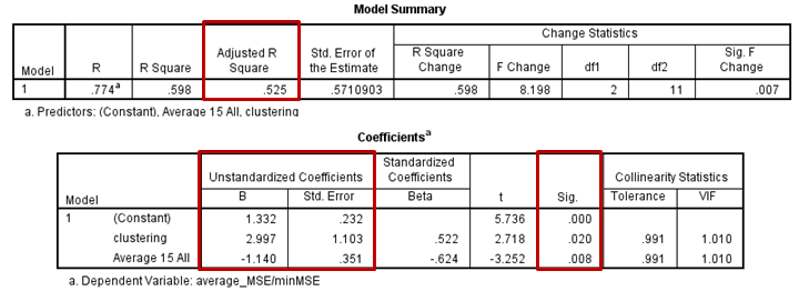
In the final model, all coefficients should be listed as significant. Record the Adjusted R Square value for the model. Multiplying this value by 100% will indicate the percent of the variance in the independent variable that is explained by the predictors in your final regression model. Further, record the coefficient B values, standard errors, and their associated significance. The B values indicate the degree to which each predictor is either positively or negatively correlated to the dependent variable in the final model. Assessing these relationships can yield information about how changes in each independent variable effect the dependent variable, which can be used to evaluate model performance and consider biological implications. A significant model for db2 in which average MSE:minMSE ratio is the dependent variable is provided below. One conclusion that could be drawn from this model is that GRNmap is best able to fit a node's expression when it is upregulated (optimized production is therefore high). Conversely, when degradation is the dominant part of a node's dynamics, it is harder for GRNmap to model that node's expression.
