Physics307L:People/Dougherty/Notebook/071112

Cary M. Dougherty 18:36, 20 November 2007 (CST)

Electron Spin Resonance

Linh and I tackled the Electron Spin Resonance. The entire lab was simple except for the setup which was fairly complicated. After the setup we were able to take date a very easily and were able to get decent data.

The purpose of the experiment is to observe electrons subject to and outside magnetic field. then calculate the famous [math]\displaystyle{ g_s }[/math] factor.

Setup/Procedure

The setup for this experiment was complicated but after that it was very simple. The lab manual was the only tool we had in starting this experiment.

Last Year's Manual See pages 54-63

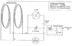
Although it may look complicated, once the circuit is set up correctly it is simple afterwards.

As seen in Fig. 1 from the lab manual, the circuit is complicated, but if broken into pieces it is easier. First, the coils are connected in parallel. Second, the DC power and the Transformer from the Variac are also connected in parallel. Next, the capacitor is connected (with correct polarity) in series with the DC power and the transformer. Lastly, one of the ends of the coil goes directly into the phase shifter and into the negative side of the DC power, while the other side of the coil goes through an anmeter and into the positive side of the DC power. The phase shifter is connected directly into channel 1 of the oscilliscope.

Half way and next is the probe and ESR adapter.

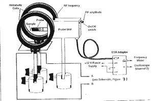
As Seen in Fig. 2 of the lab manual, the ESR is plugged directly into channel 2 of the oscilliscope and also into the frequency meter.Then it is also plugged directly into the probe. Also we hooked up the ESR to the positive end of a power supply and to a negative end of a different power supply. then connected the 2 power supplies together by the open positive and negative connections.

Also looking at Fig. 2, we can see a coil connected to the probe with a sample in it. We used 3 different types of coils with the sample during our experiment.

We then placed the coils a radius apart and placed the probe in between. We also made sure the coils were as parallel as possible by eye.

Channel 1 of the oscilliscope read the magnetic field of the coils while the probe was in the center. While channel 2 read the RF frequency within the probe.

While the probe was in between the coils we adjusted the curren and/or the frequency until we saw small spikes occur in a patter. Then we calibrated the oscilliscope so that the spikes viewed, see Fig. 3, were on the zero line of the scope. After that we used the phase shifter to sync the magnetic field of channel 1 with the spikes viewed on channel 2. (refer to lab manual because spikes may look different with each coil.) Once we had the spikes and mag. field symmetric, we took our data with different frequencies, and then used the other 2 coils and did the same.

Equipment

type w5mt3 variac autotransformer
fluke 111 true rms multimeter
homemade transformer
homemade phase shifter
soar model ps-3630 dc power supply
2x's leybold didactic gmbh helmholtz coils n=320 diam=.15m
514 55 esr-grundgerat esr basic unit
tektronix tds 1012 oscilloscope
514 56 esr addapter
HP 721A power supply x2
dpph electron source

Data

for the first 2 coils, we had not calibrated the scope so the spikes were at zero. this is crucial to read the correct frequency and current. so the data i will use for my data analysis will come from round 2 of the first 2 coils and the regular data from the last coil.

Freq:80mhz

Current: 1.231A

freq:70mhz

current: 1.130

Large Coil

range 13-30mhz

A

freq=13 mhz

Current-.238A

ch1 60mhz

ch2 undef

B

freq 17 mhz

current- .247 A

C

freq 21 mhz

current: .337 A

D

freq 25

Current: .356 A

E

freq 28

current: .481

Data Analysis

^{SJK 22:28, 9 December 2007 (CST)}

22:28, 9 December 2007 (CST)
This is pretty hard to follow without the Excel sheet! But good work you and Linh blazing the trail on this apparatus.

[math]\displaystyle{ h\nu = g_s \mu_B B \, }[/math]

[math]\displaystyle{ B = {\left ( \frac{4}{5} \right )}^{3/2} \frac{\mu_0 n I}{R} }[/math]

[math]\displaystyle{ I\; }[/math] = coil current, in amperes

[math]\displaystyle{ R\; }[/math] = coil radius, in meters = 0.135 m

[math]\displaystyle{ n\; }[/math] = number of wire loops in one coil = 320

[math]\displaystyle{ \mu_0\; }[/math] = is the permeability constant ([math]\displaystyle{ 1.26 \times 10^{-6} Tm/A }[/math])

[math]\displaystyle{ \mu_B\; }[/math] = [math]\displaystyle{ 9.2740 \times 10^{-24} J T^{-1} }[/math]

[math]\displaystyle{ \nu\; }[/math] = frequency

[math]\displaystyle{ g_s\; }[/math] = constant

[math]\displaystyle{ h\; }[/math] = planck's constant [math]\displaystyle{ 6.626 \times 10^{-34} J s }[/math]

Small Coil

A

[math]\displaystyle{ B }[/math] = 2.477*10^-3 T

[math]\displaystyle{ g_s }[/math] = 2.163

B

[math]\displaystyle{ B }[/math] = 2.959*10^-3 T

[math]\displaystyle{ g_s }[/math] = 2.172

C

[math]\displaystyle{ B }[/math] = 3.462*10^-3 T

[math]\displaystyle{ g_s }[/math] = 2.167

D

[math]\displaystyle{ B }[/math] = 3.954*10^-3 T

[math]\displaystyle{ g_s }[/math] = 2.169

E

[math]\displaystyle{ B }[/math] = 2.631*10^-3 T

[math]\displaystyle{ g_s }[/math] = 2.173

Medium Coil

A

[math]\displaystyle{ B }[/math] = 1.65*10^-3 T

[math]\displaystyle{ g_s }[/math] = 2.171

B

[math]\displaystyle{ B }[/math] = 9.531*10^-4 T

[math]\displaystyle{ g_s }[/math] = 2.249

C

[math]\displaystyle{ B }[/math] = 1.282*10^-3 T

[math]\displaystyle{ g_s }[/math] = 2.229

D

[math]\displaystyle{ B }[/math] = 1.953*10^-3 T

[math]\displaystyle{ g_s }[/math] = 2.195

E

[math]\displaystyle{ B }[/math] = 2.415*10^-3 T

[math]\displaystyle{ g_s }[/math] = 2.071

Large Coil

A

[math]\displaystyle{ B }[/math] = 5.086*10^-4 T

[math]\displaystyle{ g_s }[/math] = 1.826

B

[math]\displaystyle{ B }[/math] = 5.279*10^-4 T

[math]\displaystyle{ g_s }[/math] = 2.301

C

[math]\displaystyle{ B }[/math] = 7.202*10^-4 T

[math]\displaystyle{ g_s }[/math] = 2.083

D

[math]\displaystyle{ B }[/math] = 7.608*10^-4 T

[math]\displaystyle{ g_s }[/math] = 2.348

E

[math]\displaystyle{ B }[/math] = 1.028*10^-3

[math]\displaystyle{ g_s }[/math] = 1.946

standard error of the mean

[math]\displaystyle{ s = \sqrt{\frac{1}{N-1} \sum_{i=1}^N (x_i - \overline{x})^2} }[/math]

s = 0.0171181757

[math]\displaystyle{ SE = \frac{s}{\sqrt{N}} }[/math]

[math]\displaystyle{ SE }[/math] = 0.004419894

[math]\displaystyle{ g_s }[/math]

 [math]\displaystyle{ g_s }[/math] = 2.1509 +/- 0.00442

Physics307L:People/Dougherty/Notebook/071112

Cary M. Dougherty 18:36, 20 November 2007 (CST)

Electron Spin Resonance

Setup/Procedure

Equipment

Data

Small Coil

A

Round 2

B

Round 2

C

Round 2

D

Round 2

E

Round 2

Medium Coil

A

Round 2

B

Round 2

C

Round 2

D

Round 2

E

Round 2

Large Coil

A

B

C

D

E

Data Analysis

standard error of the mean

[math]\displaystyle{ g_s }[/math]

Navigation menu

Search