Beauchamp:ECogAnalysisV2
Beauchamp Lab wiki
|
To search for things on the wiki, use Google's site search feature. For instance, to find an Experiment Sheet, type
site:openwetware.org/wiki/Beauchamp ExperimentSheet
The eCog data analysis steps are described here. Analyzed data files for each experiment and subject can be found in /Volumes/data/lab/MUGE/
The first step is to define the "S" data structure. To do this we run generateOBJSetting.m script.
An example can be found in: /Volumes/data/lab/eCog-mfiles
Here are the components of the S data structure:
                fileName: {'YAODatafile017'  'YAODatafile018'}
             chanDesList: {1x68 cell}
                  images: 8
              imageNames: {6x1 cell}
                 kStimOn: 80
               kImageMin: 4096
    kResponse_leftbutton: 128
   kResponse_rightbutton: 129
                      Fs: 2000
               startTime: 0
              sampleTime: 0.5000
         trialTimeCourse: [1x8000 double]
Here are what the elements of the data structure represent:
- filename: Name of the raw data file. Each session of an experiment is recorded in a separate datafile.
- chanDesList: List of electrodes written according to the montage.
- images: Number of different stimuli (conditions) presented in this experiment.
- kStimOn: Stimulus onset. The onset of each presented stimulus is registered as an event. Stimulus onset events are always denoted by 80.
- kImageMin: Denotes the first stimulus. Every stimulus has a code number but the code number for the first stimulus is always 4096. 4097 denotes the second stimulus, 4098 denotes the third stimulus etc.
- kResponse_leftbutton: Left mouse button presses are registered as 128.
- kResponse_rightbutton: Left mouse button presses are registered as 129.
- Fs: Sampling frequency. The data is recorded at 2000 Hz.
- startTime: Start time of the recording.
- sampleTime: Time between each sample point (1/Fs) in milliseconds.
- trialTimeCourse: Time course of trial. e.g. -1:1/S.Fs:4 (A 5 second trial that consists of 8000 sample points).
- Data files:
Information about data files (i.e which experiment session is recorded under which data file) and electrode montage can be found in the physiology file of each subject. e.g. /Volumes/data/UT/YAO/YAOPhysiology.docx
Data files of each subject are found on the server: e.g. /Volumes/data/UT/YAO/eCog/
Data for each channel is recorded in a separate file: e.g. YAODatafile021_ch90.mat ( Data file 21, channel 90)
Audio signal (stimulus sound) is always saved in Channel 129.
A photo diode that is attached on the screen of the presentation computer during the presentation of the stimuli. It detects whenever a new video stimulus appears on the screen. This diode signal is always saved in Channel 130.
The next step is to load the appropriate data files and adjust the epochs based on the trial onset times. To do this we run the Preprocessing1.m script.
An example can be found in: /Volumes/data/lab/eCog-mfiles
This script contains the following steps:
- Loading data files:
Creates a matrix called 'traces' and saves each channel data to one row of this matrix. Audio and diode signals are saved to the last two rows of the matrix.
- Common Average Re-referencing (CAR) (Optional):
CAR calculates average over all channels (averages rows in 'traces' matrix) at each time point and subtracts that average from each individual channel.
- Classifying trials:
Trial onset, trial end, trial type and button press press information are saved in a time stamp file. e.g. /Volumes/data/UT/YAO/eCog/YAODatafile021_timeStamp.mat
'timestamp' file includes 'eventData' file. In eventData file, 4096, 4097, 4098 etc. denotes different stimuli while the following 128 or 129 denotes the behavioral response of the subject to the stimulus. For each trial we assign a number that denotes the stimulus type and response combination. Then we save these number in a separate matfile called 'imageIndex'.
- Calculating sound and video onset for each trial:
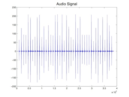
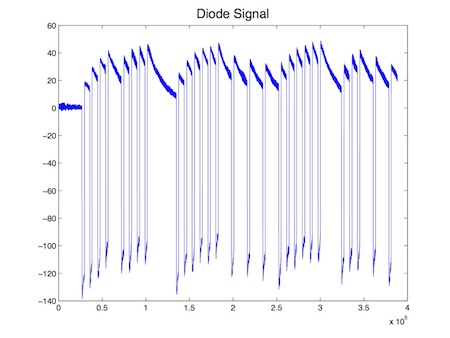
Start time of each trial is earlier than the start time of the actual stimulus (appearance of sound or video of the presentation screen). We visualize the audio signal and diode signal by plotting the 129. and 130. rows of the 'traces' matrix. We find an amplitude threshold for the audio signal such that at times the audio signal is above that threshold a sound stimulus is being presented. We also find an amplitude threshold for the diode signal such that at times the diode signal is above that threshold a video stimulus is being presented. This way we calculate the audio and video onset of each trial in an experimental session.
Here is an example of how the audio and diode signals for a whole experimental session look like :
- Epoching the signal:
'timestamp' file also includes 'eventTime' file. In eventTime file trial onset, trial end and button press times with respect to the start of the experimental session are saved (in terms of seconds). We epoch auditory only trials (i.e. trials that consist of only sound stimuli) starting from 1 second before until 3 or 4 seconds after the audio onset of that trial. We epoch visual only trials (i.e. trials that consist of only video stimuli) starting from 1 second before until 3 or 4 seconds after the video onset of that trial. Audiovisual trials can be aligned either with respect to the audio or video onset depending on the purpose of the analysis.
Next we run the Preprocessing2.m script. An example can be found in: /Volumes/data/lab/eCog-mfiles.
This script contains the following step:
- Converting data to Field Trip format:
This step defines a 'cfg' configuration structure in Field Trip format. It contains details for preprocessing options (i.e. Notch filtering). Here are the components of the cfg configuration structure:
    cfg.channel='all';
    cfg.dftfilter = 'yes';
    cfg.dftfreq  = [60; 120; 180];
    cfg.removemcg = 'no';
    cfg.precision = 'single';
Once we save the data in Field Trip format, then we run calculate_TFR.m script. An example can be found in: /Volumes/data/lab/eCog-mfiles.
This script contains the following step:
- Performing time-frequency analysis using the multi taper method. As tapers we use Discrete Prolate Spheroidal (Slepian) Sequences (DPSS).
We calculate signal power every 10 ms at 2Hz steps between 10-200 Hz. Then we perform temporal and spectral smoothing. We use Field Trip functions to perform these analyses:
    foi = 10:2:200;
    toi = -0.5:0.01:2.5;
    DF   = 10; % Width of frequency smooting: 10Hz (in every direction)
    DT   = 0.2; % Length of time window for temporal smoothing: 0.2 sec
    cfg = [];
    cfg.method = 'mtmconvol';
    cfg.output = 'pow';
    cfg.taper = 'dpss';
    cfg.toi    = toi;
    cfg.foi    = foi;
    cfg.tapsmofrq = ones(1, length(cfg.foi))*DF; % Frequency Smoothing
    cfg.t_ftimwin = ones(1, length(cfg.foi))*DT; % Temporal Smoothing
    cfg.keeptrials = 'yes';
Here is an example of how a time-frequency plot looks like:
Next we run the calculate_Gamma.m script to examine neural response at gamma band frequencies. An example can be found in: /Volumes/data/lab/eCog-mfiles.
This script contains the following steps:
- Calculating the percent signal change from the baseline:
We take 100 ms of the power signal starting from -0.5 seconds to -0.4 seconds as the baseline. We calculate the mean of the baseline over time for each channel and frequency component. Then we calculate the percent change of signal from the baseline as follows: 100 x (power signal - baseline mean) / baseline mean
- Averaging gamma band response:
For each channel and time point, we average the power signal across 70-110Hz high gamma band.
- Rejecting trials with artifacts:
We perform trial rejection analysis for each channel. For each trial, we calculate the mean and standard deviation of the gamma power across time. If at any time point gamma power exceeds mean + 6 std of the gamma power, we reject that trial.
Here is an example of how averaged gamma power response looks like:


