User:Carl Boettiger/Notebook/Stochastic Population Dynamics/2010/06/10

Stochastic Population Dynamics

Main project page Previous entry      Next entry

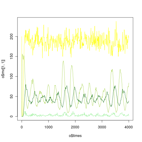
Questions Current population dynamics model macroscopic equations: [math]\displaystyle{ \begin{align} \dot E &= f_E(E,L,A) = -\mu_e E - c_{le} E L - c_{ae} E A - a_e E + b A \\ \dot L &= f_L(E, L) = -\mu_L L + a_e E - a_L L \\ \dot P &= f_P(L,P) = -\mu_P P - a_p P + a_L L\\ \dot A &= f_A(P,A) = -\mu_A A + a_p P \end{align} }[/math] Interpreting [math]\displaystyle{ \mu }[/math] terms as death events, b as birth, and the a terms as transitions between age classes gives a natural form for the master equation. Divergent Solutions to the linear noise approximation? Breaking the age classes into k subclasses makes waiting time within an age class gamma instead of exponential, which better matches observation. Also allows sustained oscillations. The numerical solution to the linear noise approximation shows divergent variance dynamics. Is this a numerical artifact? Numerical solution to linear noise b=5, ue= 0, ul = 0.001, up = 0, ua = 0.01, ae = .13*k, al = .01*k, ap = .15*k, cle = .2, cap = .1, cae = 5, V=volume version-stable code. individual base simulation with same parameters Version-stable code Differences between two-step (correlated events) and two single steps Can we distinguish between a process where an element leaves one population and enters another (i.e. a transitions from one age class to the next) and a model where death rate in one class is equal to the birth rate in another? The linear noise approximation for a two-step process obeys a different equation than the one-step: [math]\displaystyle{ \begin{align} & \frac{d}{dt} E(p) = b(p)-d(p) + \sum_{j \neq i} \tau_{ji}(p) - \tau_{ij}(p) =: f(p)\\ & \frac{d}{dt} M = \textrm{diag}( b(p) + d(p) ) - T + Df(p) M + M Df(p)^T \end{align} }[/math] where T is a symmetric matrix with off-diagonal elements i,j [math]\displaystyle{ \tau_{ij}(p) + \tau{ji}(p) }[/math] and diagonal elements chosen so that rows sum to zero. This approximation is implemented in noise_approx.R How different can this be from simply implementing all transitions as single-steps? So far the difference seems small in my examples: hastings covarainces, b1 = 0, b2 = .6, d1 = d2 = .1, c1 = c2 =.5, K =1e4 Comparison. Parameters: b_1 = .2, b_2 = .1, d_1 = d_2 = c = .1